Introduction
Estimating a proportion gets covered in virtually every introductory statistics course, so why would I be writing a post about it? There are three reasons:
- One of my goals with these posts is to explain some basic statistical concepts.
- The “standard” approach from many - possibly most - introductory books is bad.
- Especially when it is a “rare event” of interest, the standard method breaks down.
- To motivate myself to do some of the math and write a simulation comparing the alternatives so that I better understand them.
For items 2 and 3, there are some modifications and alternatives which are not really that difficult or complicated, so I think they’re suitable for a general audience (though I can see why they’re less talked about in intro stats).
To introduce some notation, let’s consider a sample of size \(n\) from an infinite population which has a proportion \(p\) of the outcome of interest, and in this sample we count \(x\) occurrences of the event of interest. For a couple of examples:
- There is a stable manufacturing process creating some component, but a certain proportion of these components will exhibit a fatal flaw. We randomly sample 100 units and count the number with the flaw. This could be either presence/absence of some defect, or pass/fail inspection on a numeric measurement.
- The CDC randomly selects a sample of 1000 individuals and counts how many of them test positive for a particular illness (influenza, COVID-19, etc).
This post will be organized as:
- Talk about the common approach usually taught in intro stats.
- Explain why that approach is not so great, for two reasons.
- Introduce two alternative approaches and explain how they arise.
- Compare the performance of the intervals.
The common approach
When an introductory statistics textbook talks about estimating a binomial proportion, they will typically say that we estimate \(p\) using \(\hat{p} = x / n\). This estimate has a sample standard error \(se(\hat{p}) = \sqrt{\hat{p}(1-\hat{p})/n}\). From this, we can construct a Wald statistic, which is asymptotically Normal, then we can use the asymptotic normality of Wald statistics to say that:
\[ \dfrac{\hat{p}-p}{\sqrt{\dfrac{\hat{p}(1-\hat{p})}{n}}} \sim N( 0, 1) \]
If we use this to set up a 2-tailed test, we can then unpack it (or “invert” the test) to obtain a confidence interval:
\[ \hat{p} \pm Z_{\alpha/2} \sqrt{\dfrac{\hat{p}(1-\hat{p})}{n}} \]
This is the confidence interval that is often (though not universally) taught in introductory statistics as the “default” or “standard.”
As a side-note, it may be easier for beginners to “see” the asymptotic normality arising as a consequence of the normal approximation to the binomial distribution. If \(X \sim \mbox{Bin}(n,p)\), then \(X \stackrel{\text{aprx}}{\sim} N( np, np(1-p) )\) under certain conditions that are not consistent from source to source. There are different ways to go about establishing this, one of which is via the Central Limit Theorem.
Common Approach: The math
If you haven’t seen the math of deriving \(\hat{p} = x / n\) and \(se(\hat{p}) = \sqrt{\hat{p}(1-\hat{p})/n}\) and would like to see, read on. If you know it already, or don’t have much calculus or probability theory background (maybe a calculus-based introductory statistics course), you may want to skip this subsection.
First we’ll derive \(\hat{p}\) using maximum likelihood estimation (MLE, which is usually pronounced M-L-E, but one prof of mine pronounced “me-lee” which was always weird to me). To do this, we take the likelihood of the data (in this case, a Binomial distribution), and find the value of \(p\) which maximizes it. Mathematically, this is just a calculus problem, and for the Binomial distribution is fairly straightforward.
The likelihood is the joint probability, but since we observe the data we think of the data as constant, and treat it as a function of the parameters of interest. In this case, the individual observations are Bernoulli (success/failure), and the joint probability is a Binomial distribution. Hence the likelihood is: \(\mathcal{L}(p|x) = \binom{n}{x}p^{x}(1-p)^{n-x}\). The typical MLE approach is to take the derivative of the log-likelihood, since that won’t move the maximum, and generally makes solving easier.
\[ \begin{aligned} L(p|X) &= \ln\mathcal{L}(p|X) = \ln \binom{n}{X} + X\ln(p) + (n-X)\ln(1-p) \\ \dfrac{\partial}{\partial p}L(p|X) &= \dfrac{X}{p} - \dfrac{n-X}{1-p} \end{aligned} \]
From there, we set the derivative to zero and solve for the parameter.
\[ \begin{aligned} 0 &= \dfrac{x}{\hat{p}} - \dfrac{n-x}{1-\hat{p}} \\ \dfrac{n-x}{1-\hat{p}} &= \dfrac{n}{\hat{p}} \\ n\hat{p} - x\hat{p} &= x - x\hat{p} \\ n\hat{p} &= x \\ \hat{p} &= \dfrac{x}{n} \end{aligned} \]
We also want the standard error of our MLE, which is just the square root of the variance.
\[ \begin{aligned} V\left[ \hat{p} \right] &= V\left[ \dfrac{X}{n} \right] \\ &= \dfrac{1}{n^2} V\left[ X \right] \end{aligned} \]
Then since \(x\) comes from a Binomial distribution, we know that \(V\left[ X \right] = np(1-p)\), substituting that in results in:
\[ \begin{aligned} V\left[ \hat{p} \right] &= \dfrac{np(1-p)}{n^2} \\ &= \dfrac{p(1-p)}{n} \end{aligned} \]
Finally, a Wald statistic is a statistic of the form:
\[ \begin{aligned} z = \dfrac{\hat{\theta} - \theta}{se(\hat{\theta})} \end{aligned} \]
where \(\hat{\theta}\) is the MLE. Since we have the MLE and its standard error, the Wald statistic is:
\[ \begin{aligned} z = \dfrac{\hat{p} - p}{ \sqrt{\dfrac{p(1-p)}{n}} } \end{aligned} \]
Then, because Wald statistics are asymptotically Normal, we use this statistic to obtain the confidence interval we saw before.
Why the common approach is bad
So why should we be looking beyond the basic approach? Because it’s bad. One way to understand that it’s bad is to look at the coverage probability of the confidence interval. If we consider the coverage probability across a range of \(p\) values, we’ll see that it often drops below the nominal value, especially so at the tails, where \(p\) is close to \(0\) or \(1\). The figure below shows the coverage probability for each \(p\) (in the interval \([0.02,0.98]\)) at a selection of sample sizes.
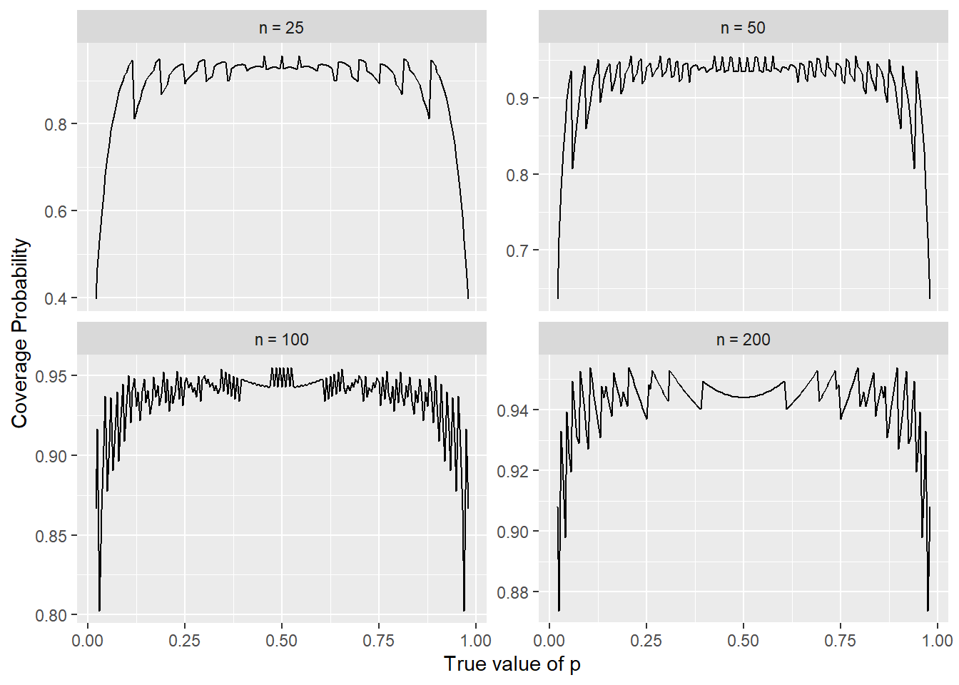
This is a similar pattern as shown in several figures from Brown, Cai, & DasGupta (2001) (which I’ll abbreviate BCD), for example, the bottom-left panel here is the same as their Figure 3, just at a different resolution. We can alternatively switch, to look at a sequence of \(n\) for a selection of \(p\).
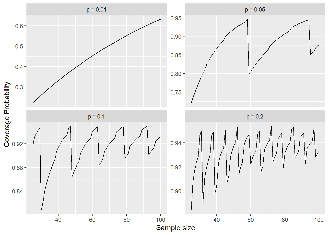
Here, the bottom-right figure is the same as their Figure 1. In both figures we see a very disturbing pattern: The coverage probability is usually below the nominal value, sometimes substantially so. Even at \(n=100\) or \(n=200\), the coverage probability rarely gets up to the nominal value for any \(p\). This is discussed in more detail in Brown, Cai, & DasGupta (2001), as well as several responses to their paper (which are included in the publication I linked above).
An in addition to that, they are very jittery. Ideally we’d like to think that the coverage probability is a smooth function, but that’s not the case here. It’s a result of the underlying discreteness of of \(X\), and there are “lucky” and “unlucky” combinations of \(n\) and \(p\).
Aside: These figures were not generated by simulation, they are exact coverage probabilities. It’s fairly straightforward to come up with the formula. For illustration, I’ll just pick a certain value of \(p\), say \(p=0.20\). We need to know the probability that, when \(p=0.20\), the confidence interval we compute will actually contain the value \(0.20\). But \(p\) isn’t what the confidence interval formula uses, right? Even if we know that \(p=0.20\), there are many possible values for \(\hat{p}\), which mean there are many possible values of the endpoints for the confidence interval. So to calculate the coverage probability, what we do (or what I did), was:
- Set up a vector \(X\) which contains the values \(0, 1, ..., n\). This is the sequence of “successes”.
- For each, compute \(\hat{p} = X/n\).
- From \(\hat{p}\), compute the endpoints of the confidence interval.
- For each confidence interval, determine whether the true value of \(p\) has been captured.
- Identify the bounds of \(X\) which result in “successful” confidence intervals. That is, determine \(X_{max}\) and \(X_{min}\), the largest and smallest values of \(X\) which produce a confidence interval which captures \(p\). For example, when \(p=0.20\), if \(X=60\) and \(n=100\), then the CI is \((0.504, 0.696)\), which does not capture \(p\).
- Compute the probability that \(X\) is contained in the interval \([X_{min}, X_{max}]\). Since we know \(p\), this is just a binomial probability: \(P( X \leq X_{max} ) - P( X \leq X_{min}-1 )\). Note we subtract 1, because \(X_{min}\) is a valid value, so \(X\) needs to be strictly below \(X_{min}\) for the interval to fail.
- Repeat steps 1-6 for a sequence of \(p\) from some “small” value to some “large” value (as indicated, I chose \(0.02\) to \(0.98\)).
Developing this idea and creating the code to produce a plot like the above would probably be a good exercise for a low-level statistics course that includes a probability component.
Alternatives
Now that we’re all convinced that the standard approach has some deficiencies, what are some alternatives? I’m going to talk about three, though two are very similar. For each I’ll try to provide a more intuitive overview, and then as before, dig into a bit of the math.
Alternative 1: Wilson and Agresi-Coull intervals
There are two (very similar) intervals I’ll mention. BCD call them the Wilson interval, and the Agresti-Coull interval. The idea is to use a slightly modified estimator in place of \(\hat{p}\):
\[ \tilde{p} = \dfrac{X + \dfrac{\kappa^{2}}{2}}{n + \kappa^{2} } \]
In this, in part to reduce notation, I’ve used \(\kappa = Z_{\alpha/2}\), which is what BCD did.
This may look weird, but it’s actually not that strange. Notice that the general form \(X/n\) is still present, but there’s a little bit added to each. And notably, it’s adding precisely half as much to the numerator as to the denominator. The effect this has is like adding a few extra samples, of which half are successes and half are failures. For example, when we select 95% confidence, then \(\kappa = 1.96\) and \(\kappa^{2} = 3.84\), so we’re adding approximately 2 to the numerator, and approximately 4 to the denominator (which was the approach suggested by Agresti & Coull (1998), alternative link on JSTOR). This has an effect of pulling the estimate slightly closer to 0.5, and also prevents it from being exactly zero, which uases problems with the standard error.
Both the Wilson and Agresi-Coull approach use this as the point estimate, but the standard errors they use are slightly different.
The Wilson confidence interval uses:
\[ se(\tilde{p}) = \left(\dfrac{\sqrt{n}}{n + \kappa^{2}}\right)\sqrt{\hat{p}(1-\hat{p}) + \dfrac{\kappa^{2}}{4n}} \]
The Agresi-Coull confidence interval uses:
\[ se(\tilde{p}) = \sqrt{\dfrac{\tilde{p}(1-\tilde{p})}{\tilde{n}}} \]
where \(\tilde{n} = n+\kappa^{2}\). With \(\tilde{n}\), we could also define \(\tilde{X}=X+\kappa\) and write the point estimate as \(\tilde{p} = \tilde{X}/\tilde{n}\). So the Agresi-Coull approach is really just the standard methods after having applied this adjustment of adding an equal number of successes and failures.
Wilson interval: The math
Alright, so how do we get these estimators and standard errors? BCD aren’t really focused on the derivation, so we need to go back to the source: Wilson (1927) (alternative: JSTOR link).
Reading that, Wilson does something interesting. First, he considers the sampling distribution of the sample proportion.
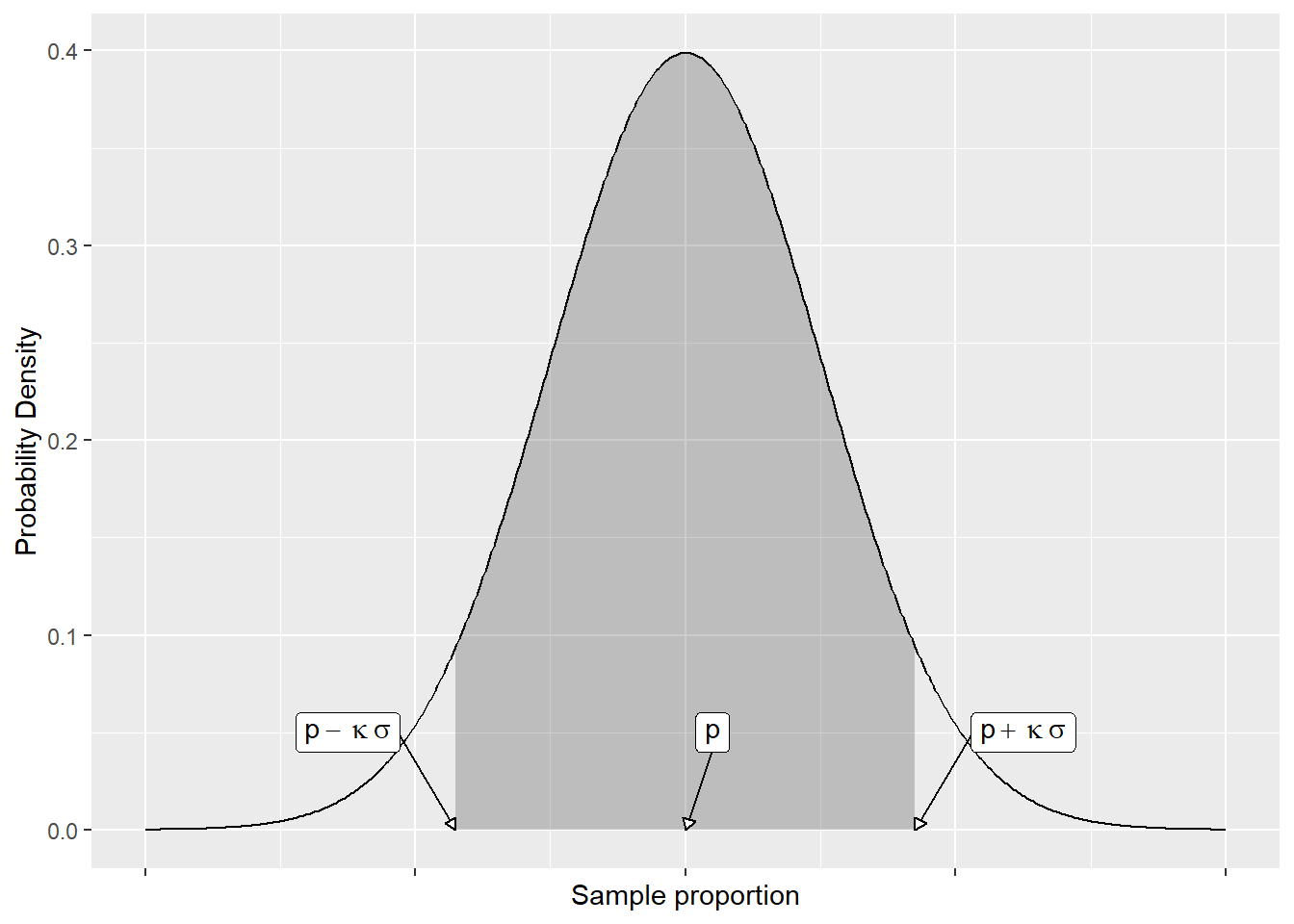
In this, \(\sigma = \sqrt{p(1-p)/n}\) and \(\kappa\) is some constant. He then points out that the probability of some value of \(p\) falling outside of the interval is \(p \pm \kappa\sigma\) is \(P( Z \geq \kappa)\). The question is then how to extract \(p\) from this. What Wilson does is square the distance between the true value \(p\) and some sample proportion \(\hat{p}\). And since we know that this distance is (with a probability determined by \(\kappa\)), we can equate the two.
\[ \left(\hat{p} - p\right)^{2} = \left(\kappa\sigma\right)^2 = \dfrac{\kappa^{2}p(1-p)}{n} \]
Small note: Wilson used \(\lambda\), I’m using \(\kappa\) because that’s what BCD used. Having set this up Wilson (probably to save notation) sets \(t = \kappa^{2}/n\), and points out that this is a quadratic expression in \(p\), so we can use the quadratic formula to solve it. We first need to expand the square, get everything on one side, and collect like terms.
\[ \begin{aligned} p^{2} - 2p\hat{p} + \hat{p}^{2} &= tp - tp^{2} \\ 0 &= p^{2}\left(1+t\right) - p\left(2\hat{p}+t\right) + \hat{p}^{2} \end{aligned} \]
Applying the quadratic formula with \(a=(1+t)\), \(b=-(2\hat{p}+t)\), and \(c=\hat{p}^{2}\) we get the solution to be:
\[ \begin{align} p &= \dfrac{2\hat{p} + t \pm \sqrt{ (2\hat{p}+t)^{2} - 4(1+t)\hat{p}^{2} }}{2(1+t)} \\ & \\ & \mbox{(some algebra)} \\ & \\ &= \dfrac{\hat{p} + \dfrac{t}{2} \pm \sqrt{ t\hat{p}(1-\hat{p}) + \dfrac{t^{2}}{4} }}{1+t} \end{align} \]
I’ve skipped a little algebra, but it’s only a couple lines at most. Once we’re here, we need to recall that \(t = \kappa^{2}/n\), and substitute that back in. I’m going to separate the fraction at the \(\pm\), and pull a \(1/n\) out from the denominator - thus multiplying the numerator by \(n\) - to cancel some of these hideous fractions-within-fractions.
\[ \begin{align} p &= \dfrac{\hat{p} + \dfrac{\kappa^{2}}{2n} \pm \sqrt{ \dfrac{\kappa^{2}}{n}\hat{p}(1-\hat{p}) + \kappa^{2}\dfrac{\kappa^{2}}{4n^{2}} }}{1+\kappa^{2}/n} \\ & \\ &= \dfrac{x + \dfrac{\kappa^{2}}{2}}{n+\kappa^{2}} \pm \dfrac{\sqrt{ \kappa^{2}n \hat{p}(1-\hat{p}) + \kappa^{2}n\dfrac{\kappa^{2}}{4n} }}{n+\kappa^{2}} \\ & \\ &= \dfrac{x + \dfrac{\kappa^{2}}{2}}{n+\kappa^{2}} \pm \dfrac{ \kappa\sqrt{n} \sqrt{ \hat{p}(1-\hat{p}) + \dfrac{\kappa^{2}}{4n} }}{n+\kappa^{2}} \\ & \\ &= \dfrac{x + \dfrac{\kappa^{2}}{2}}{n+\kappa^{2}} \pm \kappa \dfrac{ \sqrt{n}}{n+\kappa^{2}} \sqrt{ \hat{p}(1-\hat{p}) + \dfrac{\kappa^{2}}{4n} } \end{align} \]
Note that on line 2, I also multiplied the last term under the radical by \(n/n = 1\). This was to make it “match” the first term in having \(\kappa^{2}n\) that could be extracted from the radical. with this, we’ve arrived at the form of the interval I presented originally.
Remember that \(\kappa\) was defined as a quantile from the normal distribution. By expressing the solution as I have, this results has the form of a traditional normal-based confidence interval:
\[ \mbox{Estimate} \pm \mbox{Critical Value}\times\mbox{Std Error} \]
Agresi and Coull wanted to simplify this a bit, so they used the same estimator, defining:
\[ \begin{align} \tilde{x} &= x + \kappa^{2}/2 \\ \tilde{n} &= n + \kappa^{2} \\ \tilde{p} &= \tilde{x} / \tilde{n} \end{align} \]
which is adding some number of trials, evenly split between successes and failures. They then use this \(\tilde{p}\) in the “standard” form of the confidence interval. In this way they create a much better-behaving confidence interval, but which is a bit more straightforward and easier to remember than the Wilson interval.
Alternative 2: Bayesian method
Lately I’ve been going to the Bayesian approach to this problem. This might get slightly more technical if you’re at a lower mathematical level. For Bayesian analysis, we define a likelihood for the data, and a prior for the parameters. In this case, the data are Binomial, and the only parameter is the proportion, for which a Beta distribution works well. So we will assume:
\[ \begin{aligned} X | p &\sim \mbox{Binomial(n,p)} \\ p &\sim \mbox{Beta}(\alpha, \beta) \end{aligned} \]
Setting \(\alpha=\beta=1\) results in a uniform or “flat” prior, meaning we don’t have any initial judgment on whether \(p\) is likely to be large or small, all possible values of \(p\) are equally likely. Then, if we call the likelihood \(L(x|p)\) and the prior \(\pi(p)\), the posterior for \(p\) is found by:
\[ \pi(p|x) \propto L(x|p)\pi(p) \]
So, inserting the Binomial PMF for \(L(x|p)\) and the Beta PDF for \(\pi(p)\), we get:
\[ \begin{aligned} \pi(p|x) &\propto \binom{n}{x}p^{x}(1-p)^{n-x} \times \dfrac{p^{\alpha-1}(1-p)^{\beta-1}}{B(\alpha,\beta)} \\ &\propto p^{x - \alpha-1}(1-p)^{n - x + \beta-1} \end{aligned} \]
Formally, we should be performing some integration, but since we’re really interested in \(p\) here, I just want to see what the form of the resulting posterior will look like, and in this case it’s another Beta distribution, specifically, a \(\mbox{Beta}(x+\alpha, n-x+\beta)\) distribution.
With this posterior distribution, we can estimate \(p\) in several ways. We can take the mean or median as a point estimate, and we can obtain a credible interval (the Bayesian answer to the confidence interval). For example, say we had a sample of size \(n=50\), and observed \(x=1\) occurrences of the event of interest. Then taking \(\alpha = \beta = 1\) (which is a uniform prior on \(p\)), our posterior would look like below. Note that the x-axis is fairly truncated!
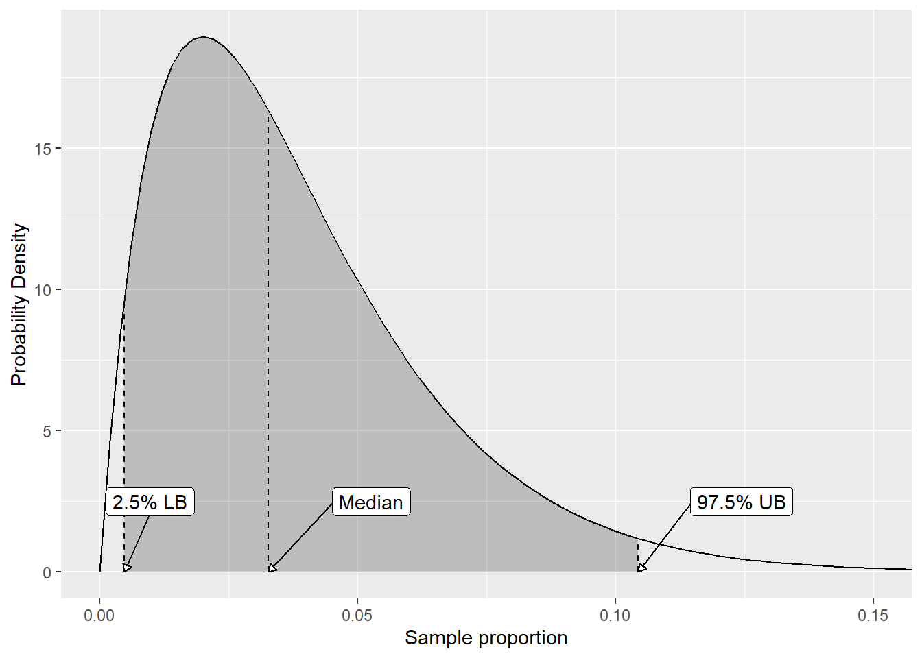
The estimate using the Wilson approach with 95% confidence, for reference, would be:
\[ \tilde{p} = \dfrac{1 + 1.96^2/2}{50 + 1.96^2} = \dfrac{2.921}{53.84} = 0.0542 \]
Comparisons
So that’s an overview of three methods for estimating \(p\) (both a point estimate and a confidence interval), but how to they compare to each other? We computed the coverage probability before, so let’s follow the same framework and compute the coverage probability for all four intervals. As before, this won’t be a simulation, but exact coverage probabilities.
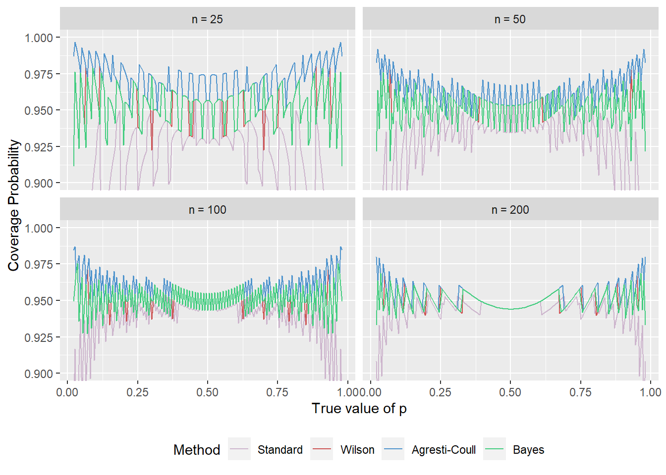
We see here again that the standard interval performs poorly, but now we can see how the alternatives stack up against it. The Agresti-Coull interval tends to have the highest coverage probability, while the Wilson and Bayes intervals are very close (being on top of each other much of the time!).
In another way of thinking about the intervals, we can consider the expected interval length. Recall when I computed the interval, I’d take a given value of \(p\) and \(n\), and compute the interval for all possible values of \(x\). So when I calculated the interval, I also obtained the length of the interval and computed a weighted average (with weight \(P(X=x)\)) of the lengths. We see that result below.
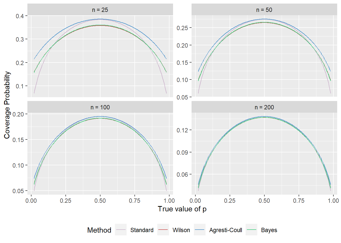
Certainly for smaller sample sizes, the Wilson and Bayes intervals produce shorter intervals (that is: more precision on \(p\)). One may be tempted to think that for small \(n\) and small \(p\) the standard interval is good here, but don’t forget the coverage probability: It drops precipitously at that point! Once we get much beyond \(n=100\) there isn’t much difference between the Wilson, Agresti-Coull, and Bayes intervals.
Summary
In this post we explored estimating a Binomial proportion, seeing how the standard method is derived, and why it’s bad, and explored some alternatives (including their derivation). Based on the coverage probabilities and interval lengths, my suggestion would be to use either the Wilson or Bayes intervals - they both have good coverage, and tend to be shorter than the Agresti-Coull interval. The Agresti-Coull has slightly higher coverage probability, but that comes at the expense of a longer interval. That being said, it depends on the behavior you want to see. The Wilson and Bayes intervals seem to have 95% coverage probability on average, while the Agresti-Coull interval seems to maintain at least 95% coverage (or very close to it) throughout.