Introduction
In a previous post I talked about estimating a binomial proportion, including for rare events. The reason I wrote that was for background to this post. Here, we’ll again be looking at estimating proportions - and can include rare events - but with an added wrinkle: A population that is finite.
In the Binomial case, every observation is assumed to be independent and have a fixed probability of the outcome of interest (a “success” or a “failure”). But when the population is finite, then the probability of success changes. One of the quintessential examples is dealing cards from a well-shuffled standard deck without replacement (that is: draw the card, and don’t put it back). Say we’re interested in the probability of getting a spade. On the first draw, this is 13/52. But the second card is either 13/51 (if the first card was not a spade) or 12/51 (if the first card was a spade), neither of which are the same as 13/52.
Sampling binary outcomes (e.g., “spade” vs “not a spade”) from a finite population gives rise to the hypergeometric distribution. This is defined as:
\[ P(X = k) = \dfrac{\binom{M}{k}\binom{N-M}{n-k}}{\binom{N}{n}} \]
where \(k \in \max(0,n+M-N)\) and
- \(N\) is the size of the population.
- \(M\) is the number of successes (or whatever event of interest) in the population.
- \(n\) is the number of samples taken.
- \(k\) is the number of successes in the sample.
What this is doing is just counting the number of ways, when drawing \(n\) samples, to get \(k\) successes.
The same situation arises in other - very practical - scenarios.
Cars have a specific year and model. Once the next “year-model” starts, no more of the previous year’s version can be manufactured. Hence, there are a finite number of, say, 2011 Chevy Cruzes available. If a problem is detected with that year-model, then the number of 2011 Chevy Cruzes which have this problem will follow a hypergeometric distribution.
For example, my own vehicle was subject to the Takata Corp airbag recall. From that wiki page, I found there were recalls of Chevy Cruze models as well.
Generalizing this idea, many components are manufactured in “batches” of some sort. That could be particular date(s) of production or batchs of raw materials. Additionally, there could be errors in the manufacturing or assembly which could potentially affect some but not all of the units produced on that day.
Estimation
When the population is finite, there are generally two possible questions of interest. Looking at the parameters of the hypergeometric distribution, this should become relatively clear: Since \(x\) and \(n\) are values from the sample (which is observed), they are fully known and not subject to uncertainty. Instead, either \(M\) or \(N\) will be the unknown quantity (hopefully not both!). In this post, I’m going to focus on the former, so the scenario can be phrased as:
For a population of size \(N\), we take a sample of size \(n\) and observe \(x\) defective units. Our goal is to estimate \(M\), the total number of defective units.
With a finite population, interest in the total number of defectives is directly related to interest in the population proportion of defectives. If we have \(M\) defectives in a population of size \(N\), then the population proportion of defectives is \(p = M/N\). So if we estimate \(M\) (perhaps with some interval bounds) we can easily convert to a proportion by dividing by the non-random population size \(N\). We could also go the other way, but \(p\) is more interpretable than \(M\), so it’s more natural to put results in terms of \(p\).
So how do we estimate the proportion? As with the case of infinite populations I discussed in my previous post, there are several approaches. One of them is the same as the “typical” approach: Divide the observed number of defectives by the sample size, \(\hat{p} = k/n\).
A wrinkle in this, however, is that when the population is finite, the samples are not independent, there is some covariance. As a result of this, the standard errors from before are no longer correct. One way of addressing this is through what’s called the Finite Population Correction Factor (FPCF).
Finite population correction factor
I think the “easy” way to see how the FPCF come about is to look at the mean and variance of the hypergeometric distribution. These are:
\[ \begin{aligned} E[X] = \mu &= n \dfrac{M}{N} \\ & \\ V[X] = \sigma^{2} &= n \dfrac{M}{N} \dfrac{N-M}{N} \dfrac{N-n}{N-1} \end{aligned} \]
Remember that the hypergeometric distribution is dealing with the number of successes (in our case, defective units), so we take \(X/n\) to deal with the proportion. This factor of \(1/n\) gets squared in the variance, so we have:
\[ \begin{aligned} E[X/n] = p &= \dfrac{M}{N} \\ & \\ V[X/n] = \sigma^{2}_{p} &= \dfrac{1}{n} \dfrac{M}{N} \dfrac{N-M}{N} \dfrac{N-n}{N-1} \end{aligned} \]
Dividing the number of defects by the sample size gets us the proportion, so in the expected value, this becomes the population proportion, \(p = M/N\), which makes sense. If we rewrite the variance in terms of \(p\), we get:
\[ \sigma^{2}_{p} = \dfrac{1}{n} p(1-p) \dfrac{N-n}{N-1} = \dfrac{p(1-p)}{n} \left(\dfrac{N-n}{N-1}\right) \]
This expression looks very close to the “ordinary” version of the standard error of \(\hat{p}\) when sampling from a Binomial distribution. There’s just an extra bit that the variance is getting multiplied by. This is the FPCP:
\[ \mbox{FPCP} = \dfrac{N-n}{N-1} \]
There is another derivation of this for a more general case (just assuming a mean and a variance), but it’s fairly long, so I don’t want to get side-tracked with that.
Bayesian estimation
As before, I’ve been interested in the Bayesian approach to this problem. There’s a paper by Jones & Johnson (2015) that talks about this (as a precursor to a more complex idea). In section 2 of their paper, they have a nice summary of the approach using a concept called superpopulation. This is a way of describing a theoretical population from which our population is drawn.
Clear as mud, right? I think of it this way: We have a population of \(N\) units, of which \(K\) are defectives (and so there is proportion \(p\) defectives). But we can consider a more general process from which our population was drawn. In this more general “superpopulation” there is some underlying proportion of defectives, which we will denote \(\pi\). With this framework, we can consider the population as being a sample of size \(N\) from the superpopulation.
The next important bit of this is that we separate the population into the observed and unobserved samples. These are effectively two independent samples from a Binomial distribution, of sizes \(n\) and \(N-n\), respectively. The diagram below is how I picture it.
In this, a solid arrow denotes the random sampling, and a dashed arrow denotes inference. So from the superpopulation we sample the population, but we conceptualize two independent samples: One which we observe, and the other which we do not. Then the observed sample is used to infer about the superpopulation, and that information about the superpopulation is used to make probabalistic statements about the unobserved sample - that is: The rest of the population.
Jones & Johnson (2015) tell that inference about \(U = M-x\) (from which we can derive \(M\), and therefore \(p\)) will make use of a Beta-binomial distribution, which I’ll denote \(betabin( N, \alpha, \beta)\). This distribution has the following PDF:
\[ P(U=k) = \binom{N}{k} \dfrac{B\left(k+\alpha, N-k+\beta \right)}{B\left(\alpha, \beta \right)}, \]
where \(B(\cdot,\cdot)\) is the Beta function (a core feature of the Beta distribution). It will be useful to see the form of this:
\[ B\left(\alpha, \beta \right) = \int_{0}^{1} x^{\alpha-1} (1-x)^{\beta-1} dx \]
The Beta distribution is obtained “simply” by dividing both sides by \(B\left(\alpha, \beta \right)\) so that the integral comes out to \(1\).
So how does the math work out? We will assuming the following likelihoods and prior:
\[ \begin{aligned} k|\pi &\sim \mbox{Bin}\left( n, \pi \right) \\ U|\pi &\sim \mbox{Bin}\left( N-n, \pi \right) \\ \pi &\sim \mbox{Beta}\left( \alpha, \beta \right) \end{aligned} \]
Then to get the distribution of \(U|k\), we can say the following:
\[ \begin{aligned} f(U|k) &\propto f(U|\pi) f(\pi | k) \\ &= f(U|\pi) \times \left[f(k | \pi) f(\pi)\right] \end{aligned} \]
The second term on the second line is mainly for clarity of what we’re doing. We already know the posterior distribution of a proportion when sampling from a Binomial distribution (since we walked through it in the previous post with infinite populations). With the likelihoods and priors denoted above, we can say that \(\pi|k \sim \mbox{Beta}( k+\alpha, n-k+\beta)\).
Now, the idea is to get at the distribution of \(U\), so conceptually we could think of doing the following (which is why the Beta-binomial can be considered a Binomial distribution for which the probability of success is unknown and randomly drawn from a beta distribution):
\[ f(U) = \int_{0}^{1} f(U|\pi) f(\pi)d\pi \]
But \(f(\pi)\) is selling ourselves short; we have more information than the prior, right? So really what we’re doing is:
\[ f(U|k) = \int_{0}^{1} f(U|\pi) f(\pi|k) d\pi \]
This allows us to take advantage of what \(k\) and \(n\) told us about \(\pi\). The dependence on \(k\) gets “inherited” from \(f(\pi|k)\). The math is below, though for ease of notation, I’m going to write \(\alpha^{*}=k+\alpha\) and \(\beta^{*} = n-k+\beta\).
\[ \begin{aligned} f(U|k) &= \int_{0}^{1} f(U|\pi) f(\pi|k)f(\pi|k) d\pi \\ & \\ &= \int_{0}^{1} \binom{N-n}{u} \pi^{u}(1-\pi)^{N-n-u} \dfrac{1}{B(\alpha^{*}, \beta^{*})} \pi^{\alpha^{*}-1} (1-\pi)^{\beta^{*}-1} d\pi & \\ &\\ &= \binom{N-n}{u}\dfrac{1}{B(\alpha^{*}, \beta^{*})} \int_{0}^{1} \pi^{u+\alpha^{*}-1}(1-\pi)^{N-n-u+\beta^{*}-1} d\pi \end{aligned} \]
If you look back to the definition of the Beta function, you’ll note that the integral here is exactly that, so we can simplify this to:
\[ \begin{aligned} f(U|k) &= \binom{N-n}{u}\dfrac{1}{B(\alpha^{*}, \beta^{*})} B( u + \alpha^{*}, N-n-u+\beta^{*}) \end{aligned} \]
This, we can note, is precisely the form of the Beta-binomial distribution. So we can say that:
\[ U|k \sim \mbox{betabinomial}( N-n, k+\alpha, n-k+\beta) \]
From the Beta-binomial distribution we can get values such as the median of \(U|x\), or quantiles to form a credible interval. Hence, the Bayesian approach offers an alternative form of point and interval estimation.
Comparison
As before, I will compare the methods computationally, using the coverage probability as the metric of interest. This will need to be a bit more elaborate, since we have added another parameter, \(N\), into the mix. As before, I’m calculating exact coverage probabilities, though now the hypergeometric distribution is used to find the probability that the number of defects is within the proper range.
Since the “standard” method was empirically worse than the others for the infinite population case, I’m no longer considering it, and will only compare the following three approaches:
- Wilson interval with FPFC
- Agresti-Coull interval with FPFC
- Bayesian interval
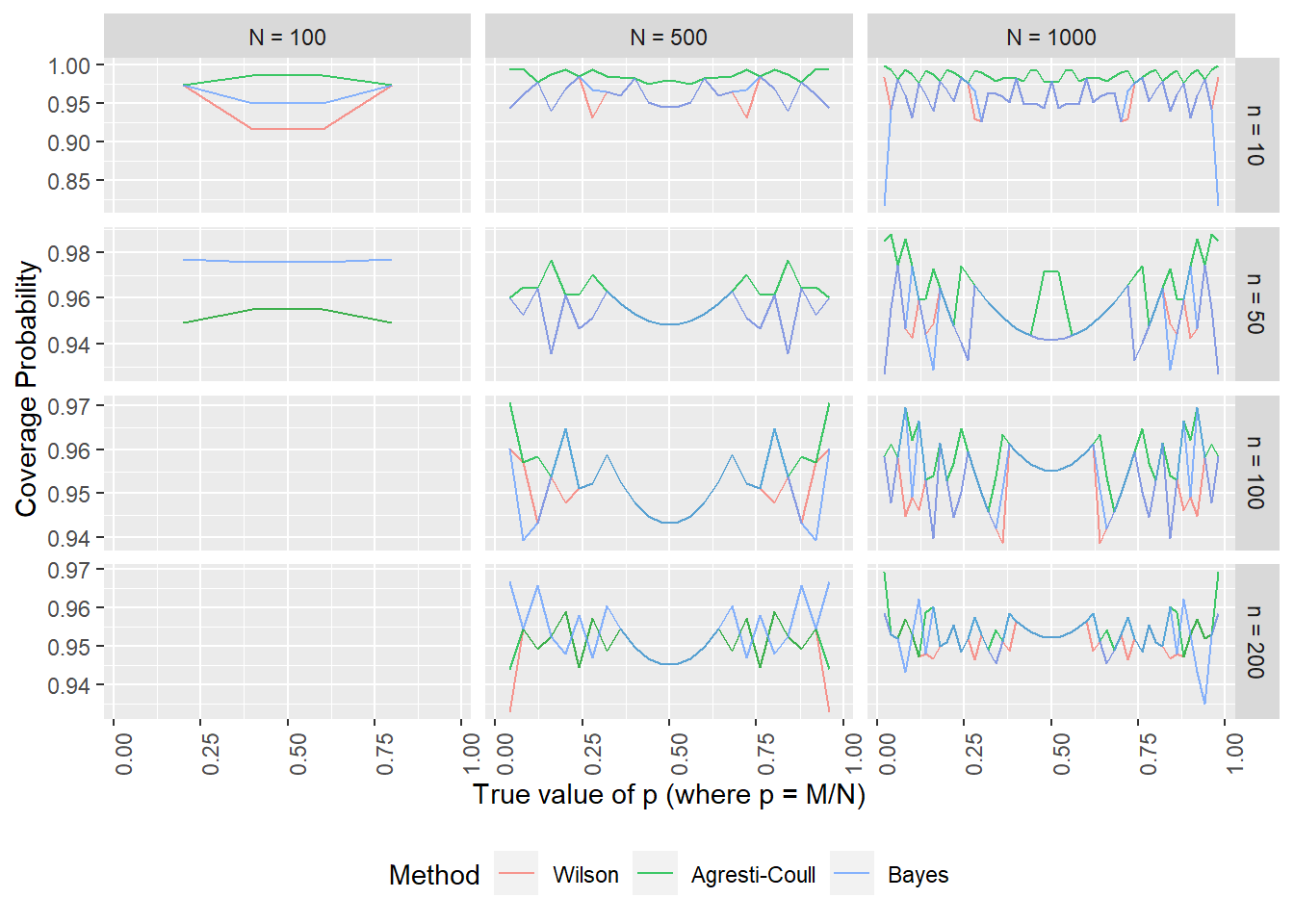
As with the infinite-population case, these three intervals behave fairly similarly, with the Agresti-Coull interval being perhaps over-conservative (wider interval) in some cases. What is interesting to me is that the Bayesian interval dropped in coverage probability when the sampling rate was small (notably, the \(N=1000, n=10\) case). This will hopefully be a fairly rare occurrence - and in my practice has been - so I wouldn’t necessarily rule out the Bayesian interval.
Summary
This was actually the post that I wanted to write, but I thought the infinite population case needed to be covered first. Maybe that’s just my inner professor coming out and wanting to build concepts from the ground up. Anyway, I hope these posts were interesting, they were for me!