Preface
For this post, I’m going to assume you are fairly familiar with RMarkdown. If not, you may want to start with RMarkdown: The Definitive Guide, or R for Data Science. The short version is that RMarkdown is a flavor of the markup language Markdown, which uses plain-text formatting and can be rendered into a variety of output types, including PDF, MS Word, HTML, and others. With RMarkdown, you can incorporate R “code chunks” to create a fully reproducible document.
With RMarkdown, you can also create a PowerPoint presentation, meaning that you can create a reproducible slide deck which includes code and results. You might ask why use PowerPoint when there are a variety of presentation formats that RMarkdown supports. I personally like the xaringan format. However, sometimes your hands are tied.
- Perhaps you’re doing an analysis for someone who insists on PP (maybe they’ll just take a couple of your slides to incorporate into a larger presentation).
- Maybe you have a corporate PP template that you have to use.
- Maybe the technology that the presentation will be projected on doesn’t support HTML slides.
- Maybe it’s something else.
So for whatever the reason, you need to make do with PowerPoint.
Another complication: Suppose you need to do the same basic analysis for a number of variables. For example, say you need to generate a set of boxplots, and a table of summary statistics for each variable in Fisher’s Iris data, comparing across the three Species. You’re already using RMarkdown, because you don’t want to be running results in R and then pasting figures and tables over to the slide deck manually. But you also don’t really want to be copy-pasting the same code all over, right? (Hint: No, you don’t). So we’d like to automate this process. You should be familiar with writing loops in R, and with that and a child document we can do exactly this.
We’ll need two files for this task, I’m going to name them main_doc.Rmd and child_doc.Rmd. The next sections will walk through the code that will go into each.
Main Document
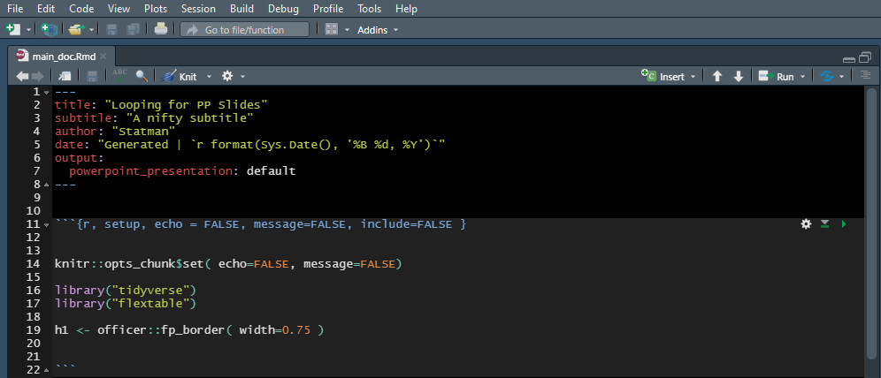
Only the main document will need a YAML header, child documents can do without (come to think of it, I’m not sure if they are allowed to have YAML headers). A basic one might look like this:
---
title: "Looping for PP Slides"
subtitle: "Presentation subtitle"
author: "Casey Jelsema"
date: "Generated | `r format(Sys.Date(), '%B %d, %Y')`"
output:
  powerpoint_presentation: default
---
Though note that I included one minorly fancy thing here, by setting the date to be a bit of R code so that it automatically updates when the file is knit. You may or may not want that. You can also put it elsewhere, for example in document type reports, I often set the subtitle to be the date.
For PP presentations, the section header (#) is what tells the document to start a new slide. You can change this with a setting in the YAML header.
For instance, maybe you will have several sections, so you want two pound signs to denote the start of a new slide, you’d add slide_level: 2 to the
output section, nested underneath powerpoint_presentation, see slide level).
There are also a variety of other options available, including setting a reference document for a custom template, or having a two-column slide.
Both of those are described here.
The rest of the main document is below. I’ll just past it all and then talk about it.
```{r, setup, echo = FALSE, message=FALSE, include=FALSE }
knitr::opts_chunk$set( echo=FALSE, message=FALSE)
library("tidyverse")
library("flextable")
```

# Introduction

In this presentation we use Fisher's iris data as an example.

```{r, load-data, results="hide" }
data(iris)
iris <- iris %>% mutate( Species = str_to_sentence(Species) )
```

- There is a code chunk here where I'm loading the data and doing some formatting to clean it up.
- For the demonstration I'm just going to loop through to make some box plots and a table for each of the variables.

```{r, loop-over-params, results="hide" }
param_vec <- colnames(iris)[1:4]
nParam    <- length(param_vec)
out <- rep(NA,nParam)
for( ii in 1:nParam ){
  param_ii <- param_vec[ii]
  param_ii_nice <- str_replace( param_vec[ii], "\\.", " ")
  out[ii] <- knitr::knit_child("child_doc.Rmd")
}
```

```{r, print-slides, results="asis"}
cat( paste(out, collapse="\n") )
```
The setup chunk, is, well, your setup chunk. I usually use that to load which packages I’ll
be using, setting options, sometimes specifying little helper functions I use, setting up a theme for
ggplots or creating linetypes for flextable. The setup chunk here is a pretty basic one.
Then the section header # Introduction gives us a first slide (well, beyond the title slide) with some comments.
Note that the code chunk if there, between the first line and the two bullet points, but we don’t see it.
If you’re familiar with RMarkdown, this shouldn’t be surprising.
The next chunk, loop-over-params is where the action is. So what am I doing?
- Get the variables to loop over, and get the number of them. Here I was easily able to extract them from the data. You might need to do a bit more work for that.
- The
outobject is setting up a container for me to put the slides for each variable, so that I’m not “growing” the object throughout my loop. - Then in the
for-loop, I’m grabbing the variable name, creating a nicer version of it for printing. - Finally, I run the child document with the command
knitr::knit_child("child_doc.Rmd").
This works because I wrote the child document with a generic param_ii, so as that object gets modified,
the child document uses different variables. The results get put into the iith space of the out container.
Finally, the last chunk here will print the results of the looping so that they are incorporated into
the document. You need to use the results="asis" option, and collapse all of the results together with
a newline.
Child Document
A basic version of the child document is here. One thing I want to draw your attention to is that none of these chunks are labeled. That’s because if they get run multiple times, RMarkdown will (appropriately!) complain that there are chunks with the same name. I haven’t tried to dynamically name the chunks yet. An quick search showed that I’m not alone in this, and there were some solutions proposed. I haven’t tried them, and have not had a need to really try.
```{r, results="asis"}
# figure-slide-title
cat("# Response: ", param_ii_nice, " | Box plots" )
```

```{r, fig.height=3.5 }
# figure-slide
ggplot( iris , aes_string(x="Species", y=param_ii) ) +
  geom_boxplot( aes(fill=Species) ) +
  labs( y=param_ii_nice )
```
The first chunk is setting the title of the slide, using the “nice” version of the parameter name.
Again, I’m printing with the chunk option results="asis", because we want to paste exactly what
we write into the Rmd. After that, I’m just making the figure. One bit you may not be familiar with
is the aes_string command in ggplot. Note that typically variable names are unquoted in ggplot.
If you have a quoted string, then aes_string will help you out here.
Then on to the table.
```{r, results="asis"}
# table-slide-title
cat("# Response: ", param_ii_nice, " | Statistics" )
```

- Comments you want to make in the child slide need to use some conditional logic.
- Otherwise the same comments go on every child slide.
- That means they should probably be rather basic, if this is supposed to be automated.

```{r, ft.left=1, ft.top=6 }
# table-slide
iris %>%
  group_by( Species ) %>%
  summarize(
    Mean = round( mean( get(param_ii) ), 2 ),
    SD   = round( sd( get(param_ii) ), 3 ),
    N    = n()
  ) %>%
  flextable() %>% theme_zebra() %>% autofit()
```
Again, I’m first defining the slide title with a results="asis" chunk option, then making the
content of the slide. I tend to use the
flextable package for tables,
though some parts of officer help to do some fine-tuning.
There are other table-making packages, but these have been more than enough for my needs.
I don’t remember exactly why I switched from using the kable function to flextable, I think that
I was having a difficult time with MS Word tables. Maybe I just didn’t put in enough effort. Regardless,
flextable has been easy for me to make tables in the formats I’ve needed, and the author is actively,
improving it, so I haven’t had a reason to look elsewhere.
In the table-slide chunk, note that there are chunk options ft.left=1, ft.top=4. These
define where the top-left of the table will be placed. It helps to arrange the content and
the output on a slide. I’m not sure if they work with tables generated from other packages.
So, if you’ve copied these code chunks into main_doc.Rmd and child_doc.Rmd (well, you can
call the first one whatever you like, but the code references child_doc.Rmd), then you should be
able to generate a slide deck that has two slides for each variable, along with a first introductory
slide.
You should be able to take it from there. Add more slides at the beginning as necessary, add more slides after looping over the variables, add more slides into the child document, make a fancier loop, or anything. Once you have the building blocks, it’s just a matter of arranging them appropriately. My hope is that this little demo gave you another building block.
Two other aspects I’d like to demonstrate are: Two-column slides; and conditional logic for dynamically generating the output comments.
Two-column slides
This one is pretty easy. As I noted above, the RMarkdown book has examples. The basic idea is that you have a set of colons (:) to denote the start and end of column sets, and a (smaller) set of colons to denote the start and end of columns, like so:
:::::: {.columns}
::: {.column width="40%"}
Content of the left column.
:::

::: {.column width="60%"}
Content of the right column.
:::
::::::
So, for instance, we might replace the table-slide with the following, we get a two-column slide.
Note that the column notation goes outside the chunk, or put another way, the code chunk goes
inside a particular column.
```{r, results="asis"}
cat("# Two-column Slide: ", param_ii_nice, " | Statistics" )
```

:::::: {.columns}
::: {.column width="40%"}
```{r, ft.left=1, ft.top=2 }
iris %>%
  group_by( Species ) %>%
  summarize(
    Mean = round( mean( get(param_ii) ), 2 ),
    SD   = round( sd( get(param_ii) ), 3 ),
    N    = n()
  ) %>%
  flextable() %>% theme_zebra() %>% autofit()
```
:::

::: {.column width="60%"}
- Comments you want to make in the child slide need to use some conditional logic.
- Otherwise the same comments go on every child slide.
- That means they should probably be rather basic, if this is supposed to be automated.
:::

::::::
You can put several tables in a single column, using multiple code chunks, so that you can set
ft.left and ft.top for each table. I’ll demonstrate that in the last section.
Conditional logic for results
In the placeholder text for the table slide, I mentioned that you’ll probably want to use conditional logic for the results, otherwise every iteration of the child slide will have exactly the same text. Let’s say we need to run an ANOVA on each outcome. Yes, there are issues with this, one of which is that you’d need to be paying attention to how many comparisons you’re making, and adjust p-values appropriately. I’m not going to worry about that for the moment.
In this part, I’ve added a bit of formatting to the tables. One thing I did was define a
border. To reduce typing, I add the command h1 <- officer::fp_border( width=0.75 )
to the setup chunk of my document. Often I define several lines of varying width
and style (e.g., a dashed line). This way I can use them in any table.
```{r, results="asis"}
cat("# ANOVA: ", param_ii_nice, "" )
```


:::::: {.columns}
::: {.column width="40%"}

```{r, ft.left=1, ft.top=2 }
iris %>%
  group_by( Species ) %>%
  summarize(
    Mean = round( mean( get(param_ii) ), 2 ),
    SD   = round( sd( get(param_ii) ), 3 ),
    N    = n()
  ) %>%
  flextable() %>% theme_zebra() %>% autofit() %>%
  border( part="header", i=1, border.top=h1, border.bottom=h1 ) %>%
  border( part="body", i=3, border.bottom=h1 ) %>%
  align( part="all", j=2:4, align="center" )
```


```{r, ft.left=1, ft.top=4 }
frml   <- as.formula( str_c( param_ii , " ~  Species" ) )
lm_out <- lm( frml, data=iris )

post_hoc <- TukeyHSD( aov(lm_out) )$Species %>%
  as.data.frame() %>%
  rownames_to_column() %>%
  rename( "Contrast" = "rowname", "Diff"="diff", "pvalue"="p adj") %>%
  dplyr::select( Contrast, Diff, pvalue ) %>%
  mutate( tpval = ifelse( pvalue < 0.0001, "< 0.0001", sprintf("%0.4f", pvalue) ) )

post_hoc %>% dplyr::select( Contrast, Diff, tpval ) %>%
  flextable() %>% theme_zebra() %>% autofit() %>%
  set_header_labels( "tpval"="p-value" ) %>%
  border( part="header", i=1, border.top=h1, border.bottom=h1 ) %>%
  border( part="body", i=3, border.bottom=h1 ) %>%
  align( part="all", j=2:3, align="center" )
```
:::

::: {.column width="60%"}
```{r, results="asis"}
# Conditional logic to build simple sentences for results
any_diff   <- any( post_hoc[["pvalue"]] <= 0.05 )
which_diff <- which( post_hoc[["pvalue"]] <= 0.05 )

if( any_diff ){
  which_contrasts <- str_replace( post_hoc[["Contrast"]][which_diff], "-", " and ")
  ndiff <- length(which_contrasts)

  bullets <- str_c( "- Pairwise comparisons conducted using Tukey's method.\n",
                    "- Significant differences in mean ", param_ii_nice, " were found between: " )

  if( ndiff==1 ){
    bullets <- str_c( bullets, which_contrasts )
  } else if( ndiff==2 ){
    bullets <- str_c( bullets, str_c( which_contrasts, collapse=" as well as " ), "." )
  } else{
    bullets <- str_c( bullets, str_c( which_contrasts[-ndiff], collapse=", " ), ", and between ", which_contrasts[ndiff], "." )
  }

} else{
  bullets <- str_c( "- Pairwise comparisons conducted using Tukey's method.\n",
                    "- There were no significant differences in mean ", param_ii_nice, " detected." )
}

cat( bullets )
```
:::
::::::
I’ll leave you to inspect the logic creating the sentences. The basic idea is to create a
string which has Markdown syntax and then print it using the chunk option results="asis". You
can get fancier, like incorporating the p-values or other results, and so on. But again, my point
here is to provide a building block so that you can use it to do things that I haven’t even thought about.
One thing about this is that the iris dataset happens to show a difference in mean between all
species and for all variables. If you want to see the logic changing the slides, either use a different
dataset (you’ll naturally need to change the analysis codes!), or when you load the data, make some
modification so that the means won’t differ. For example, you can permute one variable with the line:
iris[["Sepal.Length"]] <- sample( iris[["Sepal.Length"]] )
So that’s it for this post. I hope it will give you a nice little trick to put in your back pocket for use in some project in the future.